The Bethe Ansatz

According to the basic principles of statistical mechanics, for arbitrary temperatures, equilibrium properties are encoded in the partition function. Since the Hilbert space is spanned by the Bethe eigenfunctions, which are in turn catalogued by a set of sets of quantum numbers \(\{ \{ I \} \}\), we can formally write the partition function in the grand-canonical Gibbs ensemble with chemical potential \(\mu \in \mathbb{R}\) as

\begin{equation*} {\cal Z} = \mbox{Tr} e^{-(E - \mu N)/T} = \sum_{N=0}^\infty \sum_{\{ I \}_N} e^{-(E_{\{ I \}_N} - \mu N)/T} \end{equation*}

in which \(\{ I \}_N\) represents a proper set of quantum numbers at fixed particle number \(N\).

We shall now transform the explicit summation over all possible configurations of quantum numbers into a functional integral. In order to do this, imagine partitioning the real line for our quantum number coordinate \(x\) into `boxes' \(B_\alpha \equiv [x_\alpha, x_\alpha + \Delta x_\alpha \equiv x_{\alpha+1}]\), \(\alpha \in \mathbb{Z}\), each segment width \(\Delta x_\alpha\) being such that \(\frac{1}{L} \ll \Delta x_\alpha \ll 1\). In each such segment, for each individual eigenstate specified by our densitites l.rx, there are

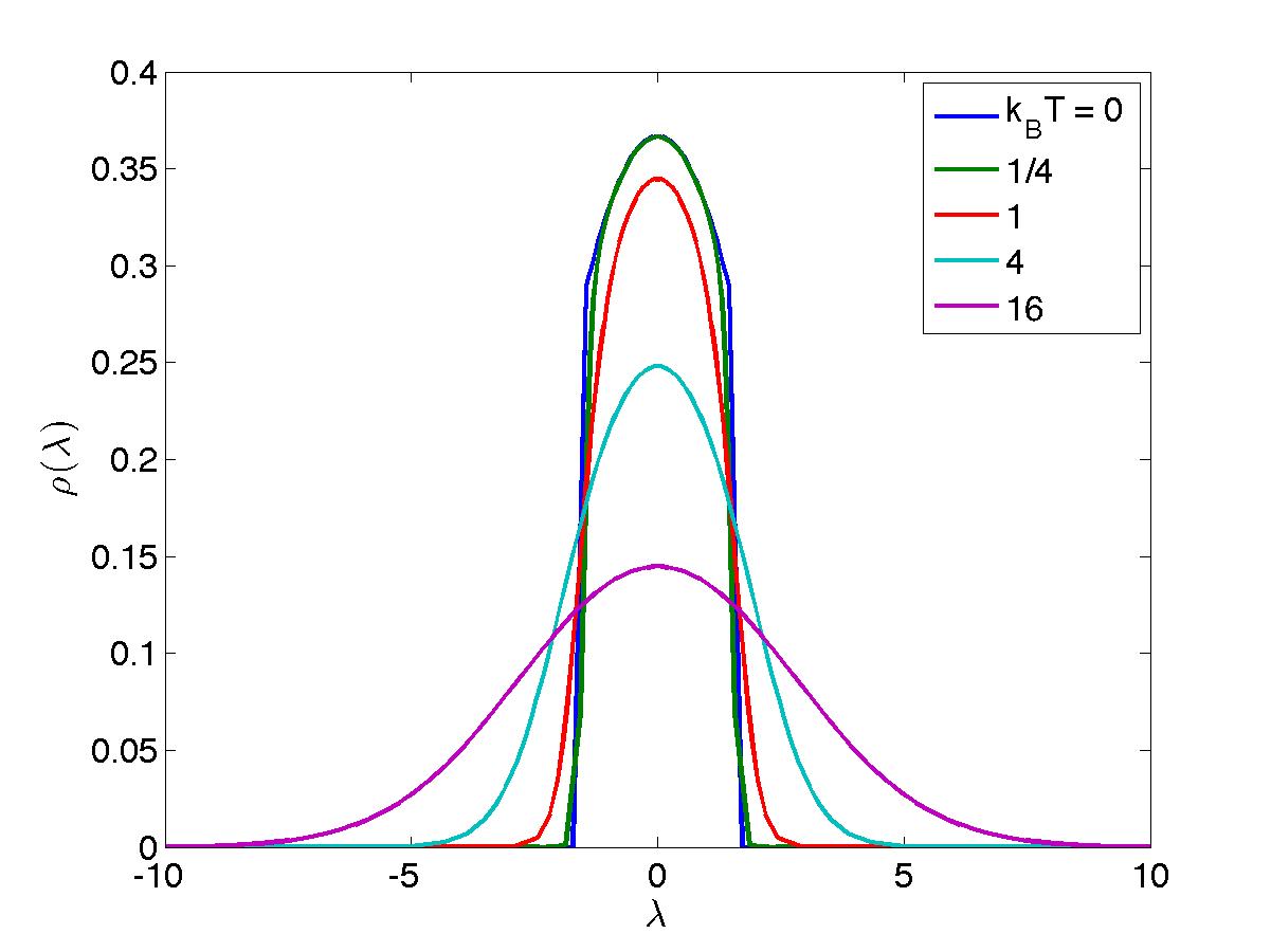
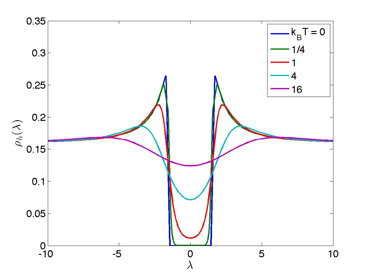
\begin{align*} L \rho_t (x_\alpha) \Delta x_\alpha ~~ &\mbox{allowed slots, with} \nonumber \\ L \rho (x_\alpha) \Delta x_\alpha ~~~ &\mbox{particles and} \nonumber \\ L \rho_h (x_\alpha) \Delta x_\alpha ~~ &\mbox{holes,} \end{align*}

where the densities obey the constraints \(\rho_t (x) = \rho(x) + \rho_h(x)\) with \(0 \leq \rho (x) \leq 1\), and \(\rho_t (x) \rightarrow 1\) upon taking the thermodynamic limit. We can then rewrite our summation over quantum number configurations as

\begin{equation*} \sum_{N=0}^\infty \sum_{\{ I\}_N} (...) = \prod_{\alpha = -\infty}^\infty ~~\sum_{n_\alpha = 0}^{L\Delta x_\alpha} ~~\sum_{\{ \frac{I}{L}\}_{n_\alpha} \in B_\alpha} (...). \end{equation*}

Let us now exploit the fact that the energy and particule number densities become smooth functionals of \(\rho(x)\) upon taking the thermodynamic limit. This means that performing "in-box" shufflings of quantum numbers in each individual segment \(\Delta x_\alpha\) does not affect the value of the Gibbs weight to leading order. As far as the partition function is concerned, we can thus write a parenthesis around the in-box summation and perform it explicitly:

\begin{equation} \left( \sum_{\{ \frac{I}{L}\}_{n_\alpha} \in B_\alpha} 1 \right) = \frac{\left[L (\rho(x_\alpha) + \rho_h(x_\alpha)) \Delta x_\alpha \right]!}{\left[L \rho(x_\alpha) \Delta x_\alpha\right]! \left[L \rho_h(x_\alpha) \Delta x_\alpha \right]!}. \tag{l.ibs}\label{l.ibs} \end{equation}

By assumption, \(\Delta x_\alpha\) is such that all numbers in square brackets are very large as compared to one. We can thus invoke Stirling's approximation

\begin{equation*} \ln (P!) = P \ln P - P + \frac{1}{2} \ln (2\pi P) + O(1/P) \end{equation*}

and rewrite the right-hand side of l.ibs as

\begin{equation*} e^{S_\alpha L \Delta x_\alpha}, \hspace{10mm} S_\alpha \equiv (\rho(x_\alpha) + \rho_h(x_\alpha)) \ln (\rho(x_\alpha) + \rho_h(x_\alpha)) - \rho(x_\alpha) \ln \rho(x_\alpha) - \rho_h(x_\alpha) \ln \rho_h (x_\alpha). \end{equation*}

Applying this logic to all boxes \(B_\alpha\) then leads us to the rewriting of our summation over quantum number configurations (provided the summand \((...)\) is blind to in-box shufflings of quantum numbers) as a functional integral weighed by an entropy functional,

\begin{align*} &\sum_{N=0}^\infty \sum_{\{ I\}_N} (...) \rightarrow \int {\cal D} [\rho(x)] e^{S[\rho(x)]} (...), \nonumber \\ &S[\rho(x)] \equiv L \int_{-\infty}^\infty dx \left[ (\rho(x) + \rho_h (x)) \ln (\rho(x) + \rho_h(x)) - \rho (x) \ln \rho(x) - \rho_h(x) \ln \rho_h(x) \right], \hspace{5mm} \nonumber \end{align*}

(note that we could simplify our expression for the entropy by using the fact that \(\rho(x) + \rho_h(x) \rightarrow 1\); we leave it as it is for later clarity), where the functional integral is viewed as the integral over the possible fillings of infinitely many boxes with in-box densities \(\rho (x_\alpha) \equiv \rho_\alpha\),

\begin{equation} \int {\cal D} [\rho(x)] (...) \equiv \lim \prod_{\alpha} \int_0^1 d\rho_\alpha (...). \tag{l.fix}\label{l.fix} \end{equation}

Our partition function is thus represented as

\begin{equation} Z \rightarrow \int {\cal D} [\rho(x)] e^{S[\rho(x)]} e^{-\frac{1}{T} (E[\rho(x)] - \mu N[\rho(x)])}. \tag{l.zx}\label{l.zx} \end{equation}

In our considerations, we have however found it convenient to work with densities in rapidity space rather than quantum number space. We can thus formally perform a functional transformation \(\rho(x), \rho_h(x) \rightarrow \rho(\lambda), \rho_h(\lambda)\) and rewrite our partition function in the grand canonical ensemble as a functional integral over the densities \(\rho(\lambda), \rho_h(\lambda)\), modulo imposition of the Bethe equations:

\begin{equation} {\cal Z} \rightarrow \int \left. {\cal D} [\rho(\lambda), \rho_h(\lambda)] e^{S[\rho,\rho_h] - E[\rho]/T + \mu N[\rho]/T}\right|_{\rho + \rho_h = \frac{1}{2\pi} + {\cal C} * \rho} \tag{l.zl}\label{l.zl} \end{equation}

where the functional integral should be read as

\begin{align*} \int {\cal D} [\rho(\lambda), \rho_h(\lambda)] &\left. (...) \right|_{\rho + \rho_h = \frac{1}{2\pi} + {\cal C} * \rho} \equiv \\ &\int {\cal D} [\rho(\lambda)] {\cal D} [\rho_h(\lambda)] ~\mbox{Det} \left[ \frac{\delta \rho(x)}{\delta \rho(\lambda)}\right] \delta (\rho + \rho_h - {\cal C} * \rho - \frac{1}{2\pi}) (...), \end{align*}

the Jacobian being interpreted as a Fredholm determinant. Note that we are being cavalier with some subtleties: the precise definition of the measures \({\cal D} [\rho(\lambda)]\) and \({\cal D}[\rho_h(\lambda)]\) parallels l.fix but has nontrivial (interaction- and state-dependent) upper limits of the individual integrals. One should thus view our version l.zl as a mere notational convenience, and see l.zx as the properly-defined version on which one should fall back in case of doubt.

The extensive particle number and energy are

\begin{equation*} N[\rho] = L \int_{-\infty}^{\infty} d\lambda ~\rho(\lambda), \hspace{10mm} E[\rho] = L \int_{-\infty}^{\infty} d\lambda ~\lambda^2 ~\rho(\lambda) \end{equation*}

and the entropy reads

\begin{equation*} S[\rho,\rho_h] = L \int_{-\infty}^{\infty} d\lambda \left( [\rho(\lambda) + \rho_h(\lambda)] \ln [\rho(\lambda) + \rho_h(\lambda)] \!-\! \rho(\lambda) \ln \rho(\lambda) \!-\! \rho_h(\lambda) \ln \rho_h (\lambda) \right). \end{equation*}

Simplifying notations somewhat, we write the partition function in the grand-canonical ensemble as the functional integral

\begin{equation*} {\cal Z} = \int \left. {\cal D} [\rho(\lambda),\rho_h(\lambda)] e^{-G[\rho,\rho_h]/T}\right|_{\rho + \rho_h = \frac{1}{2\pi} + {\cal C} * \rho}, \end{equation*}

with Gibbs weight

\begin{align*} G[\rho,\rho_h] = L \int_{-\infty}^{\infty} d\lambda \left\{ \rho(\lambda) \left[ \lambda^2 - \mu - T \ln [\rho(\lambda) + \rho_h(\lambda)] + T \ln \rho(\lambda)\right] + \right. \nonumber \\ \left. + ~\rho_h(\lambda) \left[ - T \ln [\rho(\lambda) + \rho_h(\lambda)] + T \ln \rho_h(\lambda)\right] \right\}. \end{align*}

In the limit \(L \rightarrow \infty\), this functional integral can be evaluated in a saddle-point approximation. To quantify this, we perform the variations

\begin{align*} \rho(\lambda) &\rightarrow \rho(\lambda) + \delta \rho(\lambda), \nonumber \\ \rho_h(\lambda) &\rightarrow \rho_h(\lambda) + \delta \rho_h (\lambda). \end{align*}

This gives

\begin{align*} \frac{\delta G}{L} = \int_{-\infty}^{\infty} d\lambda \left\{ \delta \rho(\lambda) \left[ \lambda^2 -\mu - T\ln[\rho + \rho_h] + T \ln \rho \right] + \rho \left[ -T \frac{\delta \rho + \delta \rho_h}{\rho + \rho_h} + T \frac{\delta \rho}{\rho} \right] \right. \nonumber \\ \left. + \delta \rho_h \left[ -T \ln [\rho + \rho_h] + T \ln \rho_h \right] + \rho_h \left[ -T \frac{\delta \rho + \delta \rho_h}{\rho + \rho_h} + T \frac{\delta \rho_h}{\rho_h} \right] \right\} \end{align*}

which simplifies to

\begin{equation*} \frac{\delta G}{L} = \int_{-\infty}^{\infty} d\lambda \left\{\delta \rho \left[\lambda^2 - \mu - T \ln [1 + \rho_h/\rho]\right] + \delta \rho_h [-T \ln [1 + \rho/\rho_h]] \right\}. \end{equation*}

The variations \(\delta \rho\) and \(\delta \rho_h\) are not independent. They are related by equation l.bec,

\begin{equation*} \delta \rho(\lambda) - {\cal C} * \delta \rho(\lambda) = -\delta \rho_h (\lambda). \end{equation*}

Substituting this in gives

\begin{equation*} \frac{\delta G}{L} = \int_{-\infty}^{\infty} d\lambda \delta \rho(\lambda) \left[ \lambda^2 - \mu - T \ln \frac{\rho_h(\lambda)}{\rho(\lambda)} - {\cal C} * T \ln \left[1 + \rho(\lambda)/\rho_h(\lambda)\right] \right]. \end{equation*}

Since this must vanish for any choice of the variation \(\delta \rho(\lambda)\), we obtain the saddle-point condition

\begin{equation*} T \ln \frac{\rho_h(\lambda)}{\rho(\lambda)} = \lambda^2 - \mu - {\cal C} * T \ln \left[1 + \rho(\lambda)/\rho_h(\lambda)\right]. \end{equation*}

We define the function

\begin{equation*} \epsilon (\lambda) = T \ln \frac{\rho_h(\lambda)}{\rho(\lambda)} \end{equation*}

whose physical meaning is to represent the energy of fundamental excitations. This gives

\begin{equation*} \epsilon(\lambda) = \lambda^2 - \mu -{\cal C} * T\ln [1 + e^{-\epsilon(\lambda)/T}], \end{equation*}

and the free energy density becomes

\begin{align*} \frac{G}{L} &= \int_{-\infty}^{\infty} d\lambda \left\{ \rho(\lambda) \left[ \lambda^2 -\mu - \epsilon(\lambda) \right] - [\rho(\lambda) + \rho_h(\lambda)] T \ln [1 + e^{-\epsilon(\lambda)}] \right\} \nonumber \\ &= \int_{-\infty}^{\infty} d\lambda \left\{ \rho(\lambda) {\cal C} * T \ln [1 + e^{-\epsilon(\lambda)/T}] - T ({\cal C} * \rho (\lambda)) \ln [1 + e^{-\epsilon (\lambda)/T}] \right\} - \frac{T}{2\pi} \int_{-\infty}^{\infty} d\lambda \ln [1 + e^{-\epsilon(\lambda)/T}]. \end{align*}

Simple manipulations show that the first two terms cancel, so we are left with the rather simple result

\begin{equation} g(\mu, T) = \frac{G(\mu, T)}{L} = -T \int_{-\infty}^{\infty} \frac{d\lambda}{2\pi} \ln \left[ 1 + e^{-\epsilon(\lambda)/T}\right], \tag{l.g}\label{l.g} \end{equation}

where the energy function is solution to

\begin{equation} \epsilon(\lambda) = \lambda^2 - \mu - {\cal C} * T \ln \left[ 1 + e^{-\epsilon(\lambda)/T}\right]. \tag{l.e}\label{l.e} \end{equation}

This encodes all the equilibrium thermodynamics of the infinite system.

Table 3: Left: the density \(\rho(\lambda)\) at \(c=1\), \(n = 1\) for various temperatures. Right: the hole density \(\rho_h(\lambda)\).