The Bethe Ansatz

The ground state is obtained through choosing the following set of quantum numbers:

\begin{equation} I_j = -\frac{N+1}{2} + j, \hspace{1cm} j = 1, ..., N. \tag{l.igs}\label{l.igs} \end{equation}

In the thermodynamic limit, we can immediately obtain an integral equation for the corresponding ground state rapidity density function. We shall look for a ground state with finite particle density \(n\). It is then natural to look for a density \(\rho_g(\lambda)\) which is nonzero only within a finite interval \(\lambda \in [-\lambda_F, \lambda_F]\) such that

\begin{align} \rho_g(\lambda) &= \left\{ \begin{array}{cc}\rho_t (\lambda), & -\lambda_F \leq \lambda \leq \lambda_F, \\ 0 & \mbox{otherwise} \end{array} \right. \nonumber \\ \rho_{g,h} (\lambda) &= \left\{ \begin{array}{cc}\rho_t (\lambda), & |\lambda| > \lambda_F, \\ 0 & \mbox{otherwise} \end{array} \right.. \tag{l.rg}\label{l.rg} \end{align}

The integral equation l.bec therefore becomes

\begin{equation} \rho_g(\lambda) - \int_{-\lambda_F}^{\lambda_F} d\lambda' {\cal C} (\lambda - \lambda') \rho_g(\lambda') = \frac{1}{2\pi}, \hspace{10mm} \lambda \in [-\lambda_F, \lambda_F] \tag{l.le}\label{l.le} \end{equation}

which is known as the Lieb equation. The Fermi momentum \(\lambda_F\) can be viewed as an independent variable which (indirectly) specifies the particle density \(n\), the relationship between these being

\begin{equation} n = \int_{-\lambda_F}^{\lambda_F} d\lambda ~\rho(\lambda). \tag{l.ng}\label{l.ng} \end{equation}

The density is a monotonically increasing function of \(\lambda_F\) for \(c>0\) (this will be proven later on), but the exact relationship cannot be written in closed form. In practice, one thus needs to solve l.le and l.ng self-consistently if one requires a specific particle density.

The Lieb equation is in fact identical to an equation known as Love's equation, occurring in classical electrostatics, and describing the capacitance of a circular capacitor. It does not admit a closed-form solution for \(0 < c < \infty\). Expansions for small or large interactions can however be written down. See b-Gaudin for details.

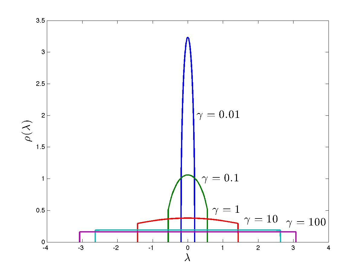
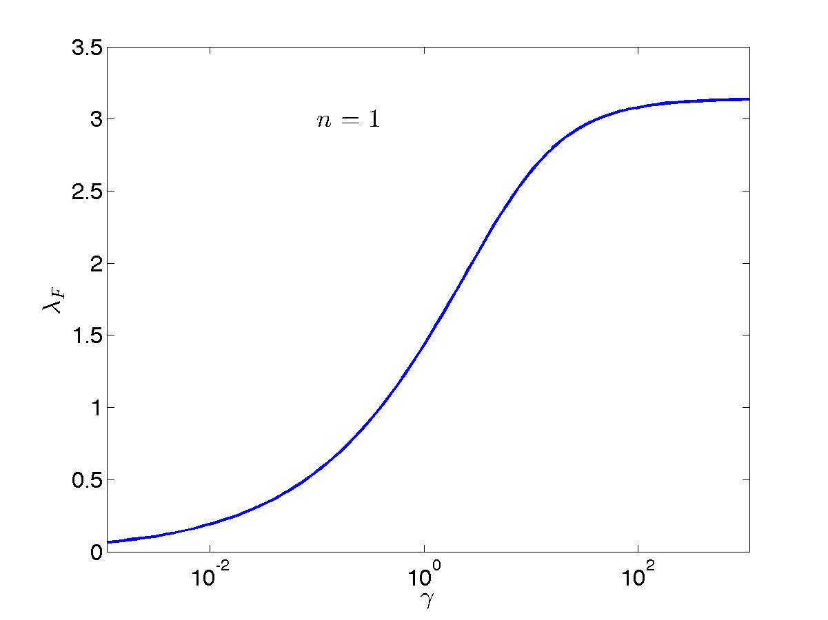
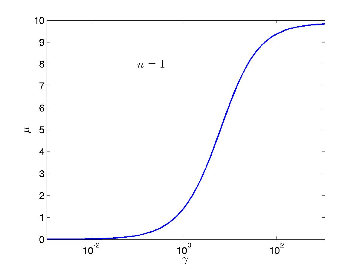
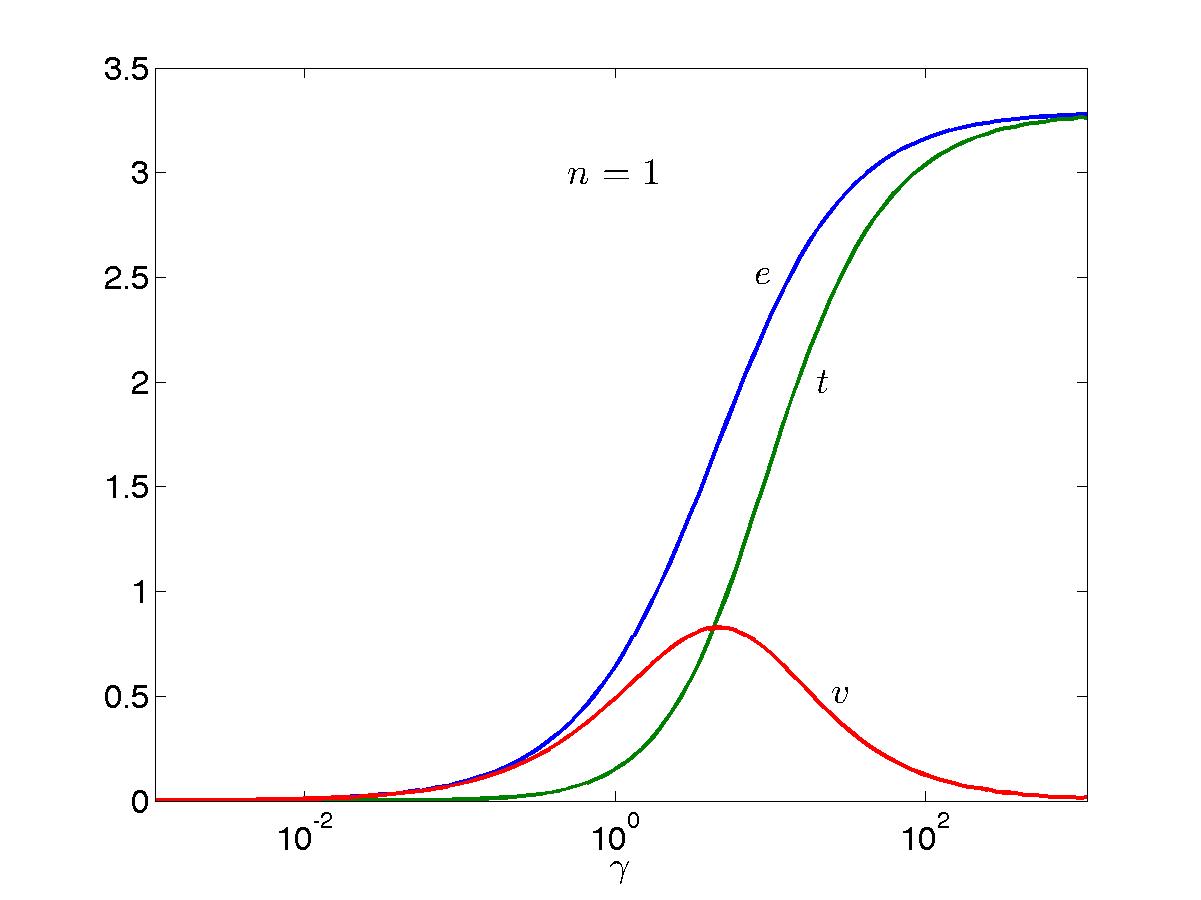
Plots of the ground-state rapidity density function \(\rho(\lambda)\) for a number of values of the interaction parameter can be found in Fig. FigLLgs. There, \(k_F\) as a function of \(c\) for unit filling \(n=1\) is also plotted, together with the chemical potential \(\mu\), as well as the total (\(e\)), kinetic (\(t\)) and potential (\(v\)) energy per unit lenght (in other words per particle at unit filling). These are simply calculated as

\begin{equation*} e = t + v, \hspace{10mm} v = c \frac{\partial e}{\partial c}. \end{equation*}

It is interesting to define the `maximally complicated' value of interaction for Lieb-Liniger as the point at which the kinetic energy density equals the interaction energy density (there is then no obvious starting point for any perturbative expansion). This occurs when \(t = v \simeq 0.82668(1)\) at \(\gamma \simeq 4.3485(1)\). Note that the interaction energy density has a maximum of \(\simeq 0.8277(1)\) at a slightly higher value of the interaction \(\gamma \simeq 4.6572(4)\), the kinetic energy density then being \(\simeq 0.8824(2)\).

Table 1: Top left: the ground state rapidity density distribution \(\rho(\lambda)\) for various values of the interaction parameter. Top right: Fermi rapidity \(\lambda_F\) as a function of interaction parameter \(c\) for unit filling \(n=1\). Bottom left: chemical potential \(\mu\) as a function of \(\gamma\). Bottom right: total (\(e\)), kinetic (\(t\)) and potential (\(v\)) energy per particle as a function of \(\gamma\).

The solution of the Lieb equation is particularly simple in the limit \(c \rightarrow \infty\), since the Cauchy kernel vanishes. One then gets

\begin{equation*} \rho(\lambda)|_{c \rightarrow \infty} = \frac{\theta (\lambda_F - |\lambda|)}{2\pi}, \hspace{10mm} \lambda_F = \pi n. \end{equation*}

The Bethe equations l.bec then give the very simple hole density \(\rho_h\) and total density \(\rho_t\)

\begin{equation*} \rho_h (\lambda)|_{c \rightarrow \infty} = \frac{\theta (|\lambda| - \lambda_F)}{2\pi}, \hspace{10mm} \rho_t (\lambda)|_{c \rightarrow \infty} = \frac{1}{2\pi}. \end{equation*}