The Bethe Ansatz

Let us here consider a one-particle excitation over the \(N\)-particle ground state, by constructing the \(N+1\)-particle state with quantum numbers

\begin{equation*} \{ I_j\} = \left\{ -\frac{N}{2}, -\frac{N}{2} + 1, ..., \frac{N}{2} - 1, \frac{N}{2} + m \right\}. \end{equation*}

This state has momentum \(P = \frac{2\pi m}{L}\), and we denote its rapidities by the set \(\{ \lambda_1, ..., \lambda_N, q \}\). As compared to the ground state rapidities \(\{ \lambda^0 \}\), the \(\{ \lambda \}\) rapidities will move by a small amount

\begin{equation*} \Delta \lambda_j = \lambda_j - \lambda_j^0 \equiv d_j/L. \label{eq:1DBG:dj} \end{equation*}

Explicitly, the Bethe equations for the ground state rapidities \(\{ \lambda_j^0 \}\) and excited state ones \(\{ \lambda_j \}\) are respectively

\begin{align*} &L\lambda_j^0 = 2\pi \left( -\frac{N}{2} - \frac{1}{2} + j \right) - \sum_{l=1}^N \phi (\lambda_j^0 - \lambda_l^0), \nonumber \\ &L\lambda_j = 2\pi \left( -\frac{N}{2} - 1 + j \right) - \sum_{l=1}^N \phi (\lambda_j - \lambda_l) - \phi(\lambda_j - q). \end{align*}

The difference \(d_j\) thus obeys the equation

\begin{equation*} d_j = -\pi - \phi(\lambda_j - q) - \sum_{l=1}^N [\phi (\lambda_j - \lambda_l) - \phi(\lambda_j^0 - \lambda_l^0)]. \end{equation*}

Since \(\Delta \lambda_j\) is of order \(1/L\), we can write

\begin{equation*} d_j = -\pi - \phi(\lambda_j - q) - \frac{1}{L}\sum_{l=1}^N \frac{2c}{(\lambda_j - \lambda_l)^2 + c^2} (d_j - d_l) + \mbox{O}(N/L^2) \end{equation*}

and therefore

\begin{equation*} d_j \left( 1 + \frac{1}{L} \sum_{l=1}^N \frac{2c}{(\lambda_j - \lambda_l)^2 + c^2}\right) = -\pi - \phi(\lambda_j - q) +\frac{1}{L}\sum_{l=1}^N \frac{2c}{(\lambda_j - \lambda_l)^2 + c^2} d_l. \end{equation*}

Inserting our definition of the density l.r, and defining the continuous function \(d (\lambda_j, q) = d_j\), we can again extend the definition of \(d(\lambda, q)\) to all \(\lambda\) by taking

\begin{align*} d(\lambda, q) &\left( 1 + 2\pi \int_{-\lambda_F}^{\lambda_F} d\lambda' {\cal C} (\lambda-\lambda') \rho(\lambda') \right) \hspace{20mm} \nonumber \\ &= -\pi - \phi(\lambda - q) + 2\pi \int_{-\lambda_F}^{\lambda_F} d\lambda' {\cal C} (\lambda-\lambda') \rho(\lambda') d(\lambda', q). \end{align*}

Introducing the displacement function for Type I particle-like excitations

\begin{equation*} D_p(\lambda, q) = d(\lambda, q) \rho(\lambda) \end{equation*}

and making use of the Lieb equation, we get

\begin{equation} D_p (\lambda, q) - \int_{-\lambda_F}^{\lambda_F} d\lambda' {\cal C}(\lambda-\lambda') D_p(\lambda',q) = \frac{-1}{2\pi} \left( \pi + \phi(\lambda - q) \right), \hspace{5mm} q > \lambda_F. \tag{l.d1}\label{l.d1} \end{equation}

The change in momentum can be expressed as

\begin{equation} \Delta P = q + \sum_{l=1}^N (\lambda_j - \lambda^0_j) = q + \sum_{l=1}^N \Delta \lambda_j = q + \int_{-\lambda_F}^{\lambda_F} d\lambda D_p(\lambda, q) \tag{l.d1p}\label{l.d1p} \end{equation}

whilst the change in free energy (so taking the chemical potential into account) is

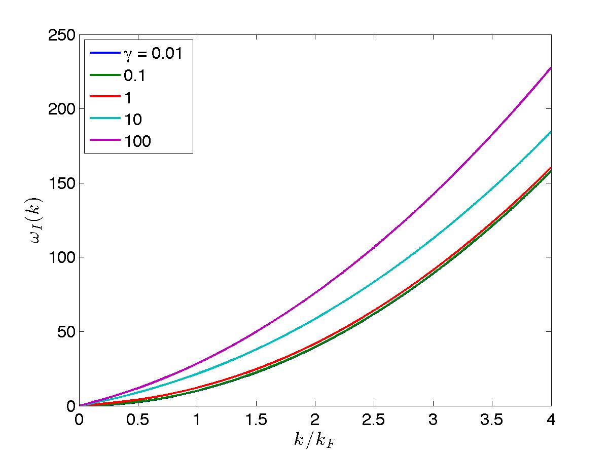
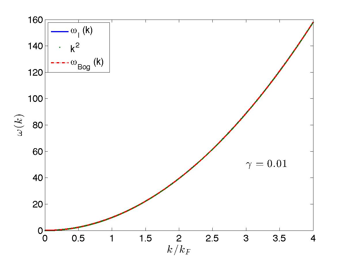
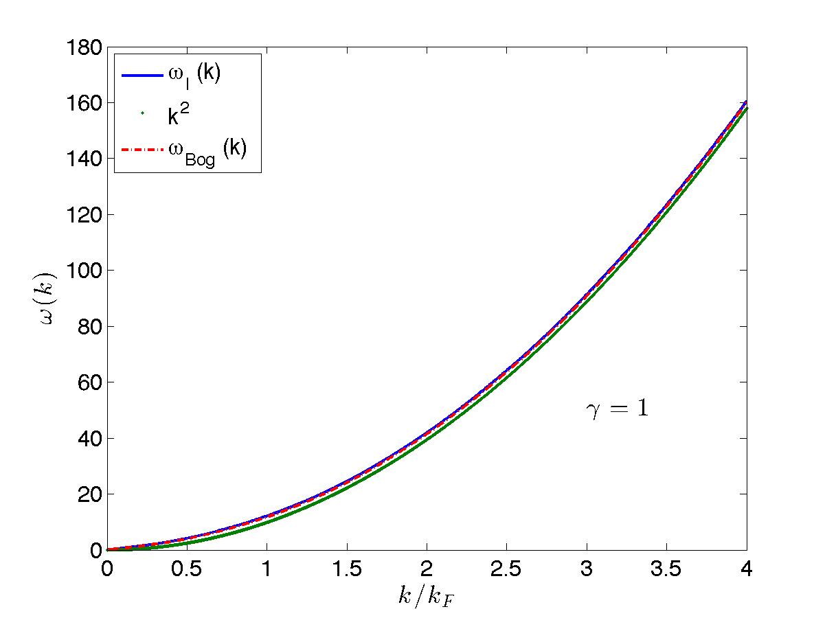
\begin{equation} \Delta E = q^2 -\mu + \sum_{l=1}^N (\lambda_j^2 - {\lambda_j^0}^2) = q^2 - \mu + 2 \int_{-\lambda_F}^{\lambda_F} d\lambda \lambda D_p(\lambda, q). \tag{l.d1e}\label{l.d1e} \end{equation}

The type I dispersion relation is illustrated in fig-T1disprel for various values of the interaction parameter, and is contrasted to the free and Bogoliubov dispersions in fig-T1comp for three values of interactions. The approximations are extremely accurate except for strong interactions.

Table 2: Comparison bewteen the exact type I dispersion curve, free dispersion \(\omega = k^2\) and the Bogoliubov prediction l.eb for three values of the interaction parameter.

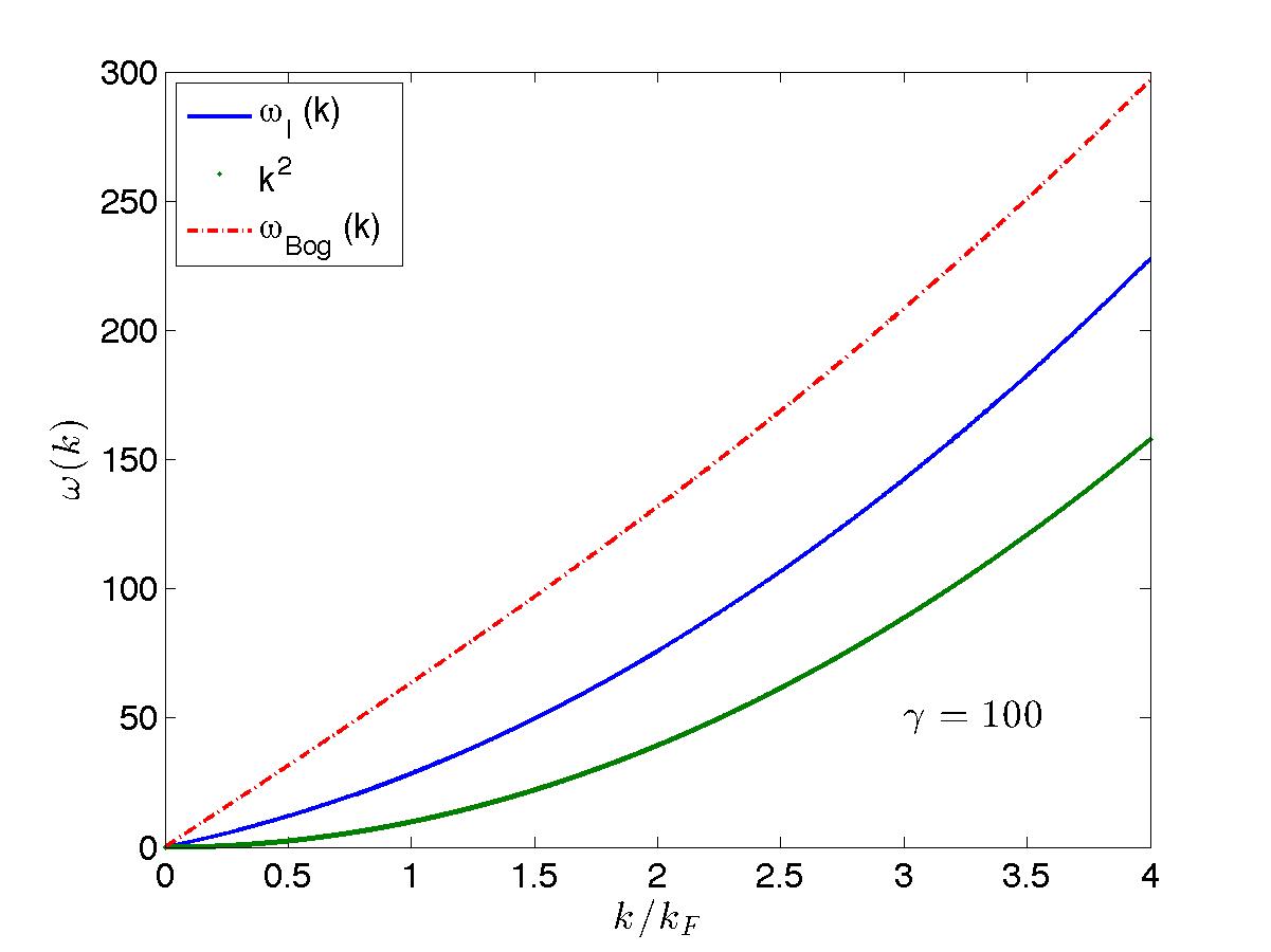In the limit \(c \rightarrow 0^+\), we get \(D_p = 0\) and thus (since the chemical potential then goes to zero), the dispersion relation for this type of excitation is

\begin{equation*} \epsilon(p) = p^2, \hspace{0.3cm} c = 0^+. \end{equation*}

For \(c \rightarrow \infty\), the solution is \(D_p = -1/2\), so \(\Delta P = q - \lambda_F\) and \(\Delta E = q^2 - \mu\). Since \(\mu = \lambda_F^2\) and \(\lambda_F = \pi n\), we obtain in this case

\begin{equation*} \epsilon(p) = p^2 + 2\pi n p, \hspace{10mm} p > 0, \hspace{0.3cm} c \rightarrow \infty. \end{equation*}

These two limits form the lower and upper limits of the particle-like excitations. Type I excitations correspond to Bogoliubov modes.