The Bethe Ansatz

Let us now do the converse of the above: we construct an excited state by starting with the \(N-1\) particle ground state, and effectivey punching a hole by moving the rightmost \(m\) particles one step to the right. Said otherwise, we set the quantum numbers to

\begin{equation*} \{ I_j \} = \left\{ -\frac{N}{2} + 1, ..., \frac{N}{2} - m - 1, \cancel{\color{grey} \frac{N}{2} - m}, \frac{N}{2} - m + 1, ..., \frac{N}{2} \right\}, \end{equation*}

where we have greyed/struck out the "hole" quantum number. For convenience, we will actually do as if the hole was participating in the Bethe equations game with its own quantum number \(I_{j=N-m}\) and its own rapidity \(\lambda_{N-m}\) which we denote \(q\) (with restriction \(|q| < \lambda_F\)). The Bethe equations for ground and excited states are

\begin{align*} &L\lambda_j^0 = 2\pi \left( -\frac{N}{2} - \frac{1}{2} + j \right) - \sum_{l=1}^N \phi (\lambda_j^0 - \lambda_l^0), \nonumber \\ &L\lambda_j = 2\pi \left( -\frac{N}{2} + j \right) - \sum_{l=1}^N \phi (\lambda_j - \lambda_l) + \phi(\lambda_j - q). \end{align*}

Subtracting these and again using the definition \(d_j \equiv \lambda_j - \lambda_j^0\) (\(j = 1, \cdots, N\)) gives (up to corrections of \(\mbox{O}(1/L, N/L^2)\))

\begin{equation*} d_j = \pi + \phi (\lambda_j - q) - \frac{1}{L} \sum_{l=1}^{N-1} \frac{2c}{(\lambda_j - \lambda_l)^2 + c^2} (d_j - d_l). \end{equation*}

Interpreting this as a continuum equation for the displacement \(D_h(\lambda,q) \equiv d(\lambda, q) \rho(\lambda)\) as we did for Type I excitations leads to

\begin{equation} D_h (\lambda, q) - \int_{-\lambda_F}^{\lambda_F} d\lambda' {\cal C}(\lambda-\lambda') D_h(\lambda',q) = \frac{1}{2\pi} \left( \pi + \phi(\lambda - q) \right), \hspace{5mm} \lambda, q \in [-\lambda_F, \lambda_F]. \tag{l.d2}\label{l.d2} \end{equation}

The change in momentum can be expressed as

\begin{equation} \Delta P = -q + \sum_{l=1}^{N-1} (\lambda_j - \lambda^0_j) = -q + \sum_{l=1}^{N-1} \Delta \lambda_j = -q + \int_{-\lambda_F}^{\lambda_F} d\lambda D_h (\lambda, q) \tag{l.d2p}\label{l.d2p} \end{equation}

whilst the change in energy is

\begin{equation} \Delta E = -q^2 + \mu + \sum_{l=1}^{N-1} (\lambda_j^2 - {\lambda_j^0}^2) = -q^2 + \mu + 2 \int_{-\lambda_F}^{\lambda_F} d\lambda \lambda D_h(\lambda, q). \tag{l.d2e}\label{l.d2e} \end{equation}

The type II dipsersion relation is illustrated in Fig. fig-T2disprel for various values of the interaction parameter.

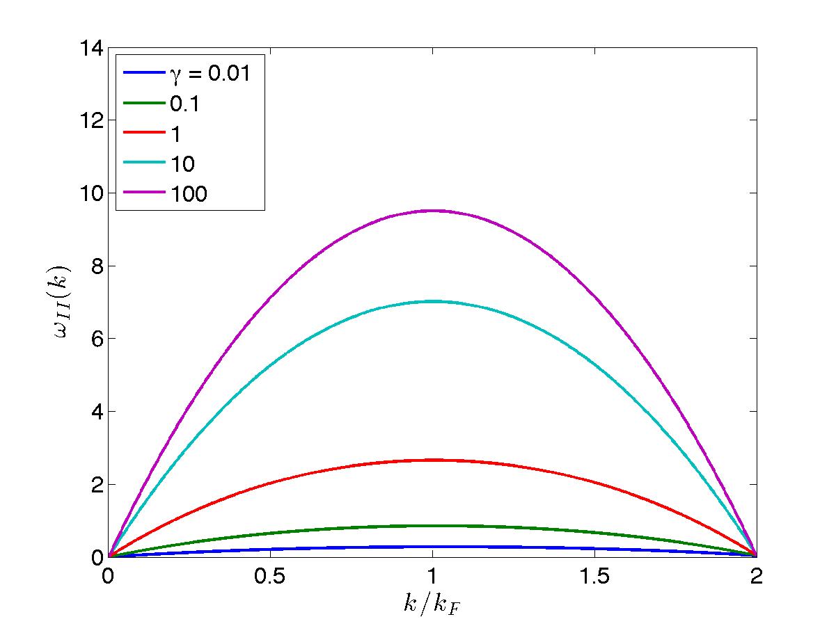
In the limit \(c \rightarrow 0^+\), we get \(\epsilon(p) = 0\).

For \(c \rightarrow \infty\), the solution is \(D_h = 1/2\), so \(\Delta P = - q + \lambda_F\) and \(\Delta E = -q^2 + \mu\). Since \(\mu = \lambda_F^2\) and \(\lambda_F = \pi n\), we obtain in this case

\begin{equation*} \epsilon(p) = -p^2 + 2\pi n p, \hspace{0.3cm} c \rightarrow \infty, \hspace{5mm} p \in [0, 2 \pi n]. \end{equation*}

These two limits form the lower and upper limits of the hole-like excitations.